Automatically create invoices from sales invoices 2 Excel (Excel)

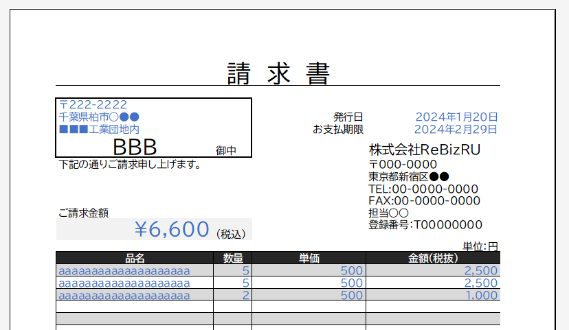
Previous.Automatically create invoices from sales invoices1 Excel (Excel)The invoicing process continues from the

Put details on invoice (use function)* Use spil

How to use the "FILTER" function

*This one uses the spill function and requires Microsoft365 or Excel 2021 or later.

This method uses the "FILTER" function.

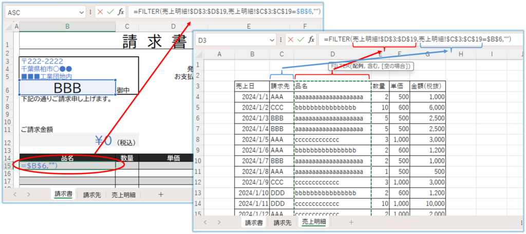
In the "B15" cell, enter this.

=FILTER($D$3:$D$19,$C$3:$C$19=$B$6,"")

."$D$3:$D$19Go to the "Sales Detail" sheet and select the key billing party column.

."$C$3:$C$19Select the column of the item name you wish to display on the "Sales Detail" sheet.

."$B$6selects the cell with the billing name on the "Invoices" sheet.

When you have finished entering the function, press the "Enter" key.

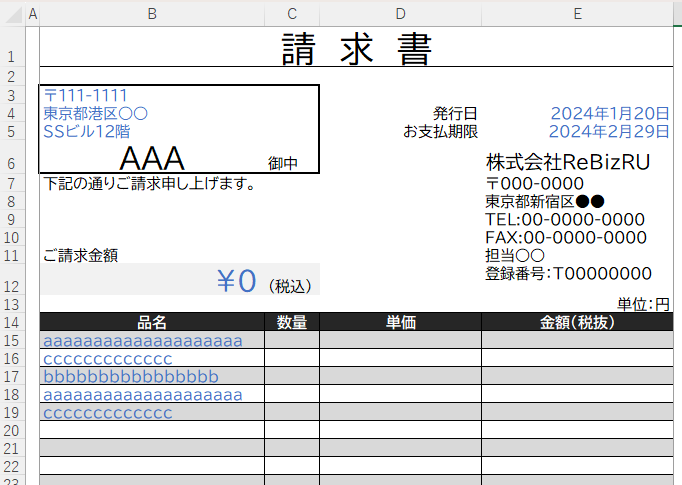
Then, even though the function was entered only in the "B15" cell, values from the "B15" cell to the "B19" cell are displayed. It should be possible to verify that this data is consistent with the sales data for the billing address of "AAA" in the "Sales Details".

Similarly, enter the "FILTER" function for the "Quantity," "Unit Price," and "Amount" columns.

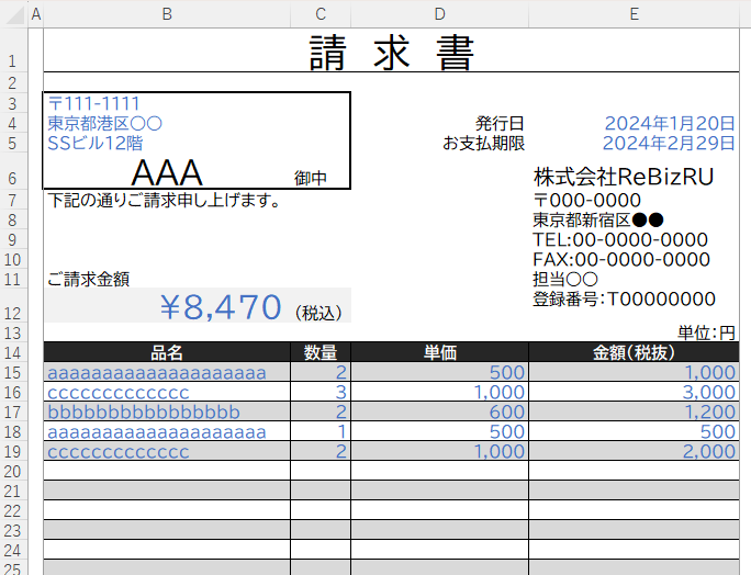
This completes the sales statement for each billing address.

Advantages of the FILTER function

• Functions are very simple and easy to create.
• Easy maintenance when changing or adding display items as you use it.

Disadvantages of the "FILTER" function

• Since it uses the spill function, it can only be handled by Microsoft365 or Excel 2021 or later. For earlier versions of Excel, the only way is to use a non-spill method or macros, which we will introduce later.
• If the number of rows to be displayed increases and the number of rows in the list is exceeded, an error will occur and all will not be displayed. If this possibility exists, a separate countermeasure should be considered.

Put details on invoices (use function) *No spiel

I don't like this approach because it is a bit aggressive, but I used to use this method when I didn't want to use macros before I was able to use spills.

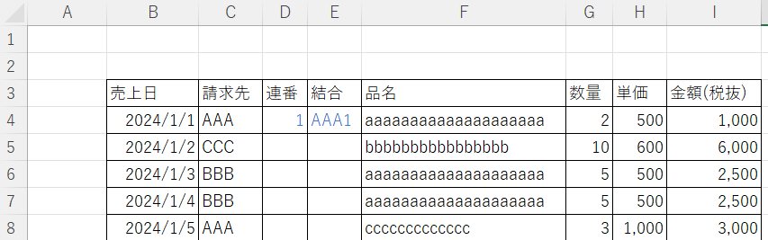
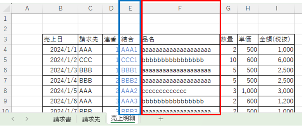
Insert columns for search keys in the "Sales Detail" sheet

I want to extract by billing address, but insert two columns next to the billing address to order them.

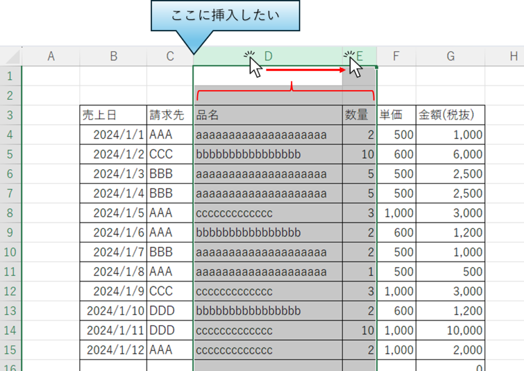
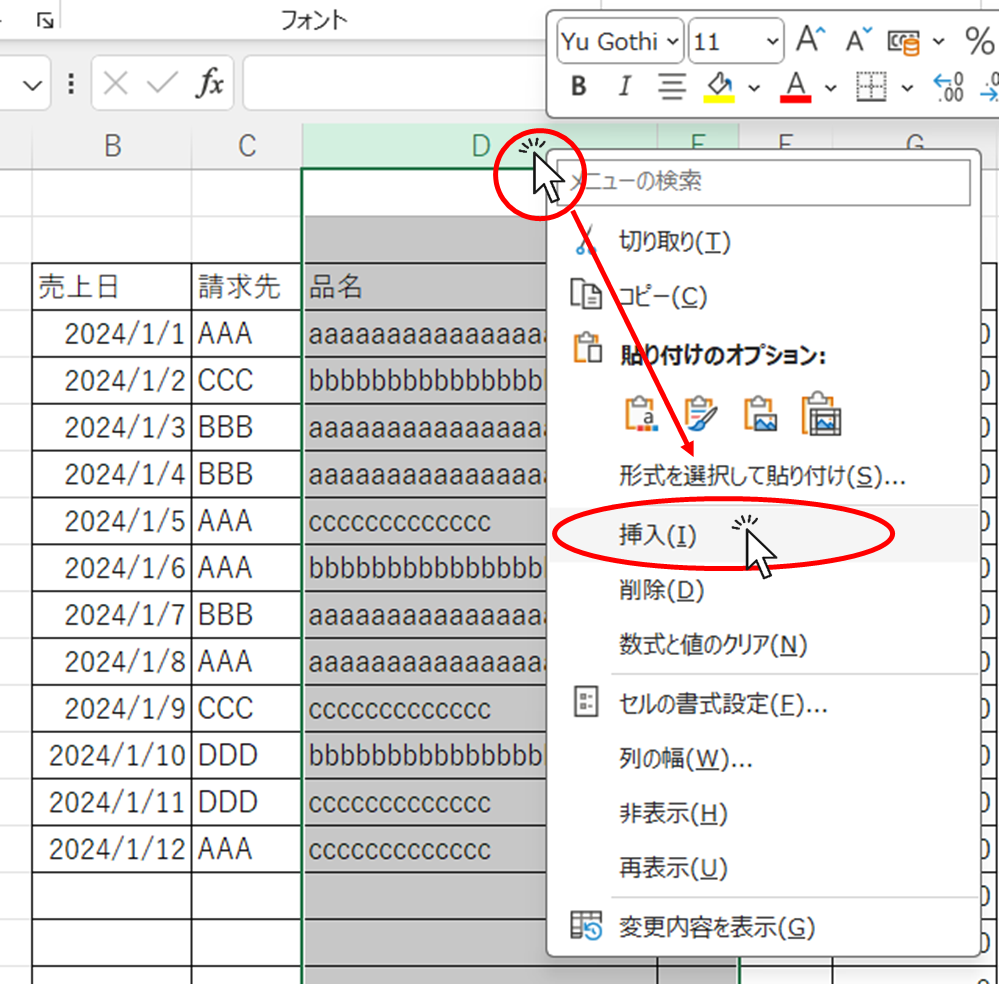
With the two columns to the right of the column you want to insert selected, "right click" → "Insert".

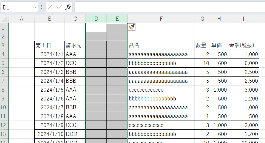
Then blank columns were inserted in columns "D" and "E".

This is not always the case, but for clarity, enter "sequential number" in cell "D3" and "join" in cell "E3".

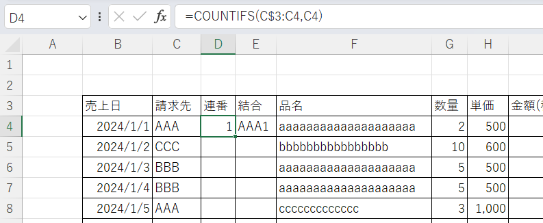
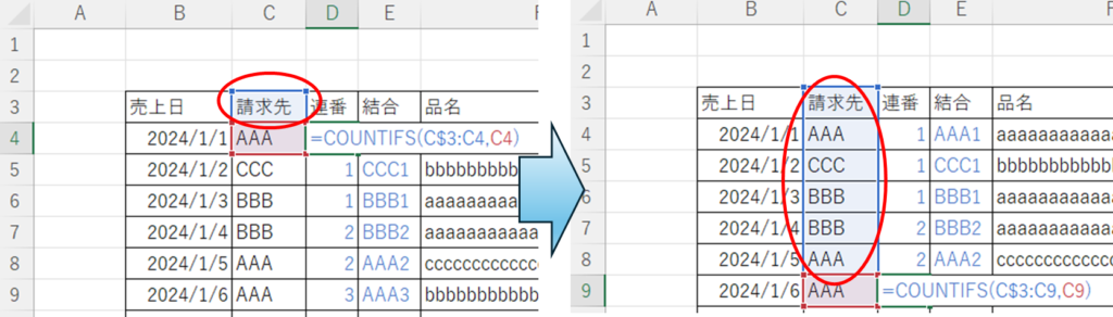
Enter the following in cell "D4". At this time, only the "3" in "C3" should be preceded by "$Please mark the "*" mark.

=COUNTIFS(C$3:C4,C4)

Then enter the following in cell "E4".

=C4&D4

Again, it is easier to understand if the cell where the function is entered is in blue.

With the "D4" to "E4" cells selected, double-click on the lower right portion.

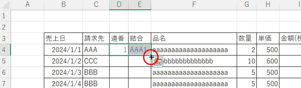
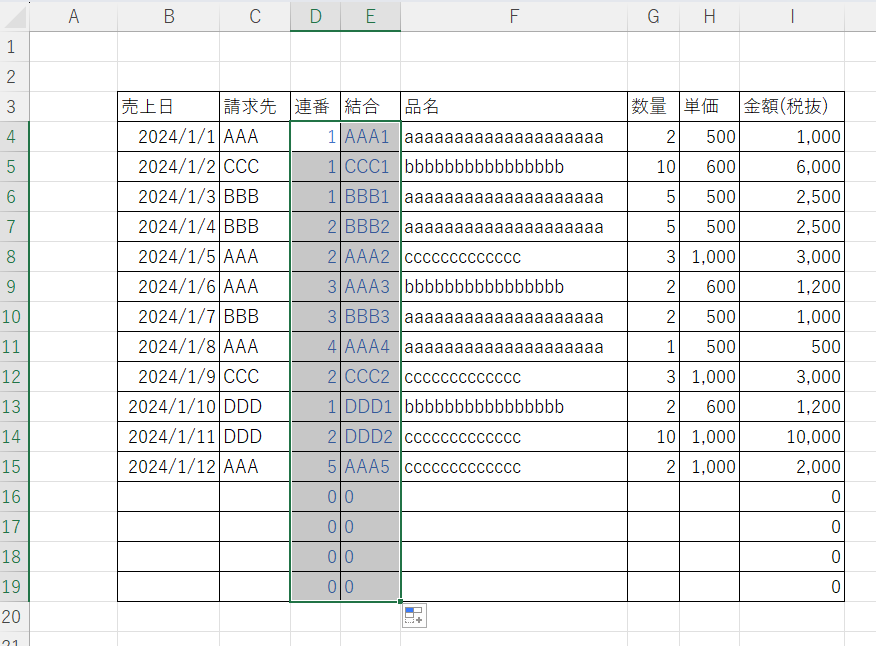
The function was then automatically entered up to the bottom line containing the data.

Comparing the functions entered in the "D4" and "D9" cells, one can see that the "$" marker has changed the range of input. This allows us to order the billing addresses if they are the same in each row.

At this point, the "Sales Detail" sheet is ready.

Display the details on the "Invoice" sheet

This section explains how to use the INDEX and MATCH functions to display the data.How to use Excel (Excel) INDEX and MATCH functions in combination

This function should be placed in cell "B15" on the "Invoices" sheet.

=INDEX(Sales details!F:F,MATCH($B$6&ROW()-14,Sales Detail!$E:$E,0))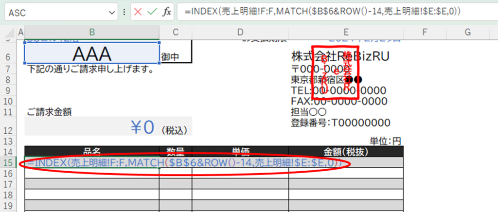

Sales details!F:Fis the column of the item name on the "Sales Detail" sheet,Sales Detail!$E:$Erefers to the key columns to search for that you just created.

Sales Detail!$E:$Eis marked "$" because it is a key column and we want other cells to refer to the same column.

$B$6&ROW()-14is the most complicated, but "$B$6" refers to the billing name, "AAA" in this case, and "ROW()-14" is the number of rows in the cell you are now entering (row 15) minus 14, which is "1".

This is connected by & to represent "AAA1". This is the same as the value in the combined column of the "Sales Detail" sheet.

Type up to this point and press "enter".

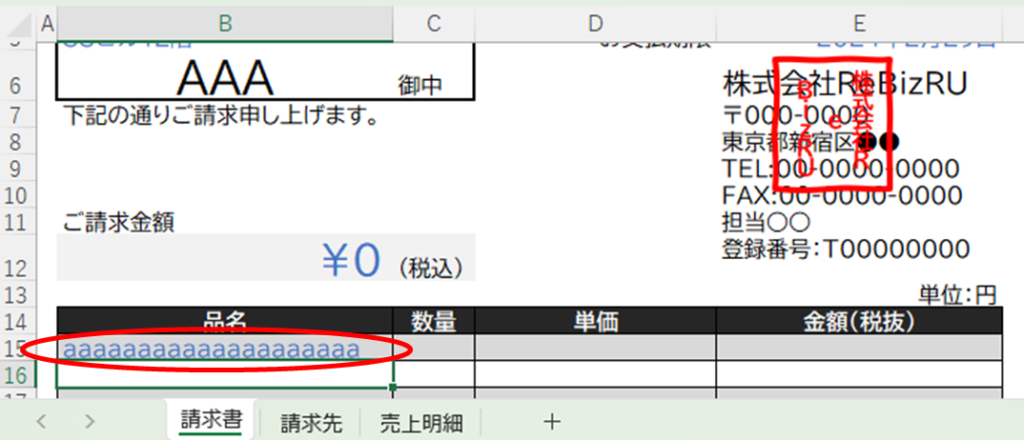
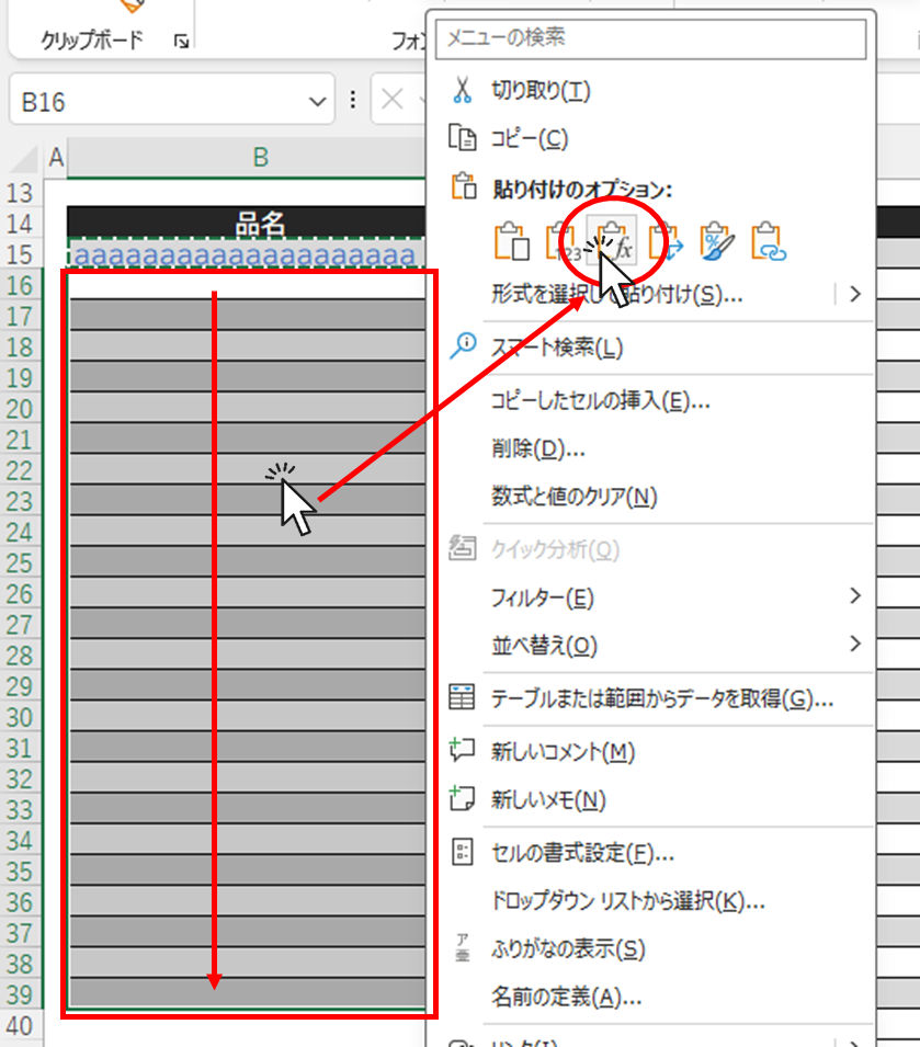
Copy the cell where you entered this formula, select the area below where you want to put the formula, and paste the "formula".

In this condition, a line with no data will return a "#N/A" error.

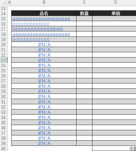
To avoid this, sandwich it with the "IFERROR" function

=IFERROR(INDEX(sales details!F:F,MATCH($B$6&ROW()-14,sales details!$E:$E,0)),"")

The meaning of this function is to return the value of the above expression if the black portion of the expression is not an error, and to return a """ space if it is an error. If there is an error, it returns a """ space. If we copy it down as well, we get

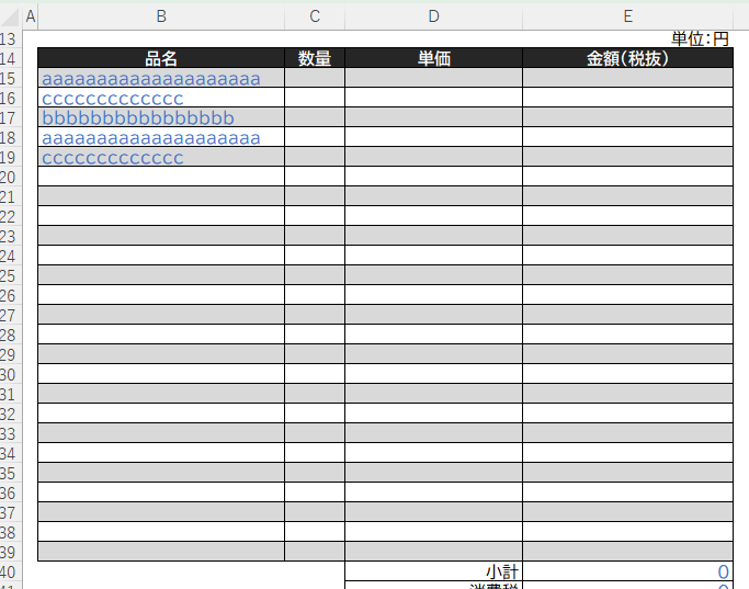
Cells with values now display values and cells without values display nothing.

Now select "B15" through "B39" in the same way and drag the bottom right square to the end of the table.

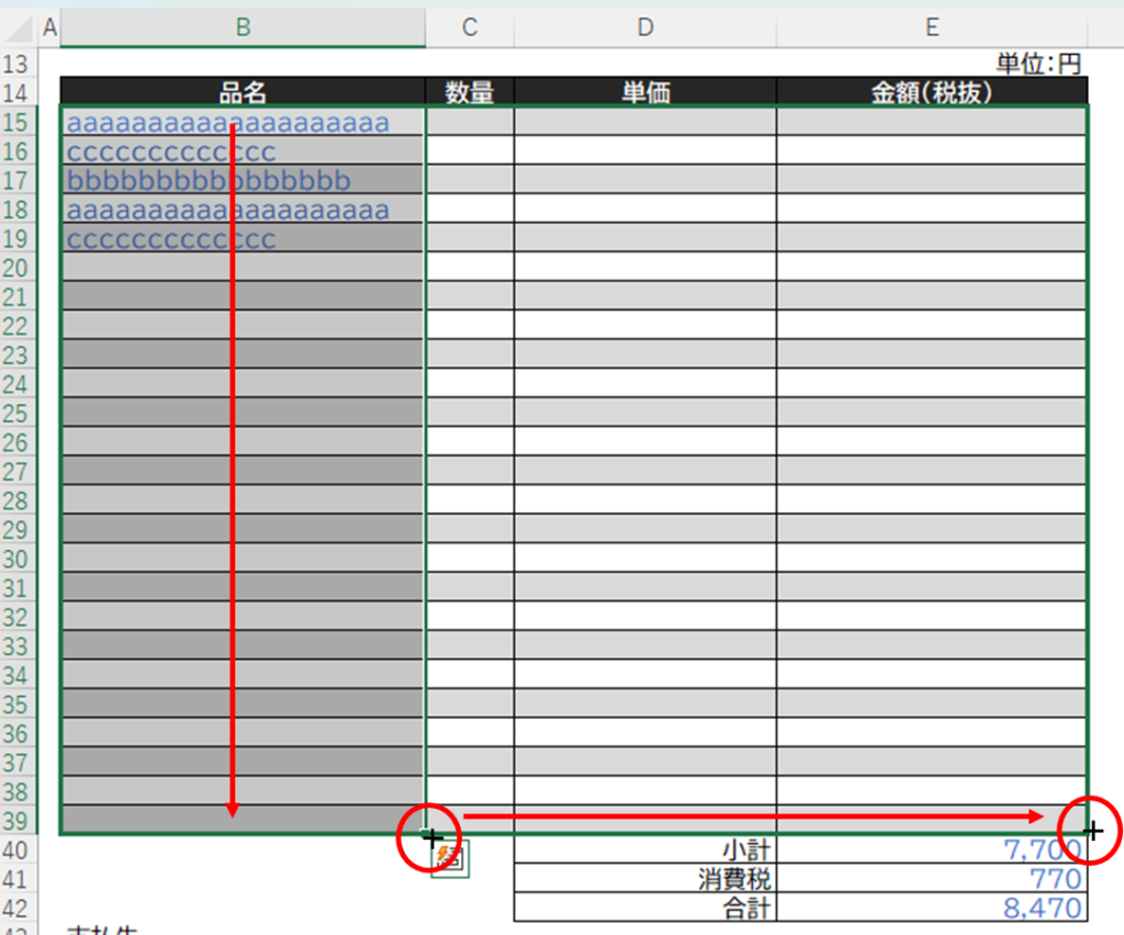
The values are then displayed correctly throughout the table.

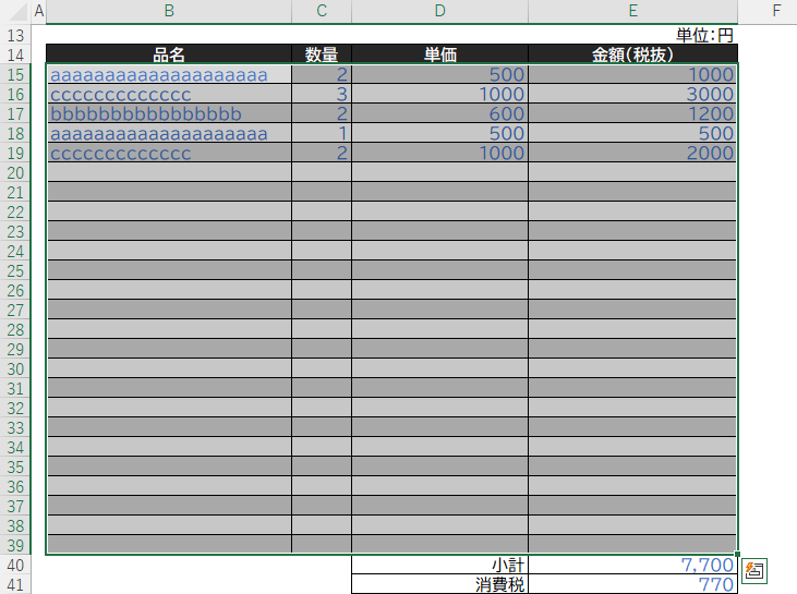
In this case, the order of the columns on the "Invoices" sheet happened to be the same as the order of the columns on the "Sales Details" sheet, so the display was correct simply by dragging the columns to the right.

Advantages of the non-spill method

• It does not use the spill function and can be used with Microsoft365 or Excel 2021 or earlier.

Disadvantages of non-spill methods

• Extra function rows are needed in the sales statement, and the function has to be copied when additional rows are added.
• If the sales detail function is broken, the invoice will not display correctly.

When using macros

This is getting a little long, so we will show you how to use macros and the final touches again next time.