
We will show you how to display the desired data by combining the INDEX and MATCH functions, which refer to data from a table on another sheet.
How to Write INDEX Functions
There are two ways to write the INDEX function.
- INDEX(array,row number,[column number])
- INDEX(reference, row number, [column number], [area number])
Since there are not many situations in which the ❷ reference setting is used, I will explain the ❶ array reference setting this time.
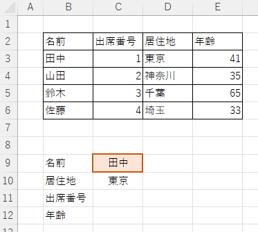
First, suppose we have a list like this. In cell "C9" we have entered "Tanaka", so we want cell "C10" to display "Tokyo" as the place of residence.

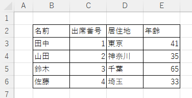
The table ranges from cell "B2" to cell "E6", and Tanaka2In line 2, the place of residence is3It is in the second column and should be listed as follows
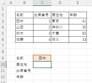
=INDEX(B2:E6,.2,3)Then "Tokyo" was displayed in the "C10" cell as shown here.
But of course, as it is, even if we change the "C9" cell, the "C10" cell will remain in Tokyo.
That is where the MATCH function comes in.
How to write the MATCH function
The MATCH function is written like this.
- MATCH(test value,test range,[collation type])
For "Collation Type," enter "1" for greater than or equal to, "-1" for less than or equal to, and "0" for an exact match.
In most cases, only exact matches are used, so set this to "0".
How to check the number of rows with the MATCH function
First, we will look at how to find the number of rows.
This time, the inspection value is "Mr. Tanaka" and the inspection range is from "B2" cell to "B6" cell that contains the name data, so if you want to know how many rows Mr. Tanaka is in the above table, you can describe it like this.
=MATCH("Tanaka",B2:B6,0)Then, since Tanaka-san is the second row in the table, the result "2" is returned.
Next, switch this ""Tanaka"" to a cell reference.

The name of the test value is entered as "C9This is a "_" cell, so it will be described as such.
=MATCH(C9,B2:B6,0)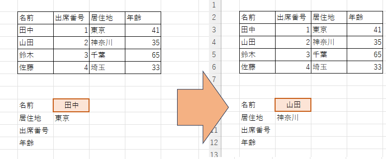
Then, when the name is changed, the place of residence also changes automatically.
How to check the number of columns with the MATCH function
We will now look at how to find the number of columns for "Residence".

This time, the test value is "Residence" and the test range is from "B2" cell to "E2" cell in the first row containing the item name, so if you want to know what column "Residence" is in the table above, you can describe it like this.
=MATCH("Residence",B2:E2,0)Then, "Residence" is the third column in the table, so the result "3" is returned.
Next, switch this ""place of residence"" section to a cell reference.
The "Residence" of the inspection value is entered as "B10", so change it like this.
=MATCH(B10,B2:E2,0)This will return a result of "3," which is the number of columns in the "Residence" column.
Next, this MATCH function is combined with the INDEX function described earlier.
How to combine the INDEX and MATCH functions
The previous INDEX function is here.
=INDEX(B2:E6,.2,3)The red 2 part represents the number of rows for Mr. Tanaka, so the MATCH function described earlier is substituted here.
The MATCH function to check the number of rows was here.
=MATCH(C9,B2:B6,0)The MATCH function to check the number of columns was here.
=MATCH(B10,B2:E2,0)Substituting these MATCH functions into the INDEX function
=INDEX(B2:E6,.MATCH(C9,B2:B6,0),MATCH(B10,B2:E2,0))The first two are the following.
Applications combining absolute and relative references
Next, rewrite the function you have just created as follows.
=INDEX($B$2:$E$6,MATCH($C$9,$B$2:$B$6,0),MATCH($B10,.$B$2:$E$2,0))You enter "$" in front of the coordinates of each matrix, but the key point is that you do not put "$" in front of the numbers as "$B10" only at "B10". This allows the reference range to move relative to the bottom of the matrix when dragging it down, rather than being fixed.
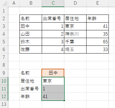
In fact, drag the lower right corner of the "C10" cell where you wrote the function to the "C12" cell.
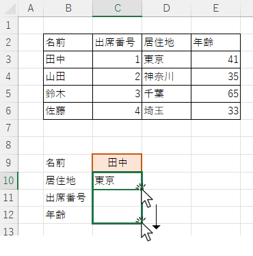
Then both attendance number and age were automatically displayed like this.
In addition, references will not be misplaced even if rows or columns are inserted in between if written in this way.
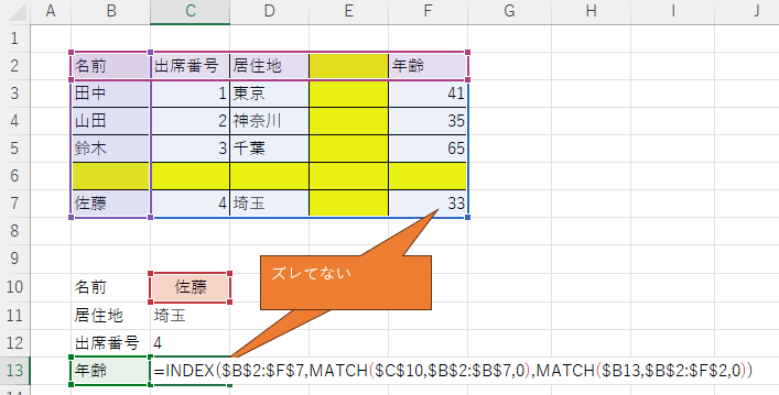
The rows and columns filled in yellow are the inserted areas.
The contents of cell "C11" also changed automatically like this.
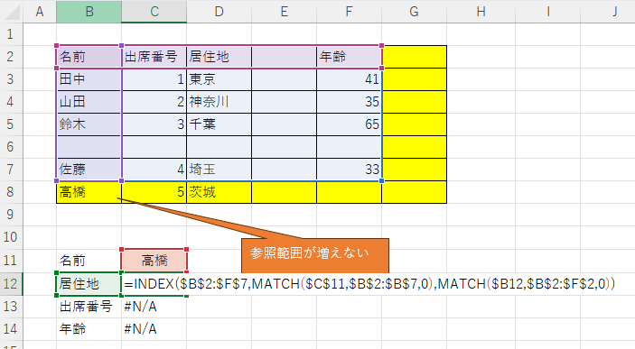
=INDEX($B$2:$f$7,MATCH($C$10,$B$2:$B$7,0),MATCH($B11,$B$2:$f$2,0))Incidentally, in this situation, matrix insertion outside of column "G" or row "8" will not increase the reference range and will result in an error.
Absolute and relative references are also explained in detail here.
Absolute and relative references in Excel (Excel)
These are the uses of the INDEX and MATCH functions.


Comment