As shown in the figure below, when the data to be extracted appears after a certain after and its length varies, the RIGHT function alone cannot extract the data.
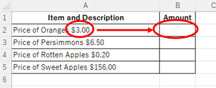
A function to extract the text after the '$' symbol in cell A2
=RIGHT(A2,LEN(A2)-FIND("$",A2))In the next sections, we will explain how this function works.
Before specific characterThe method to extract theHow to extract characters before a specific character "LEFT and FIND functions in Excel".
How to use the RIGHT function
The RIGHT function is a function that extracts XX characters from the right side of a cell string.
= RIGHT(string,[number of characters])
Both full-width and half-width characters are counted as one character.
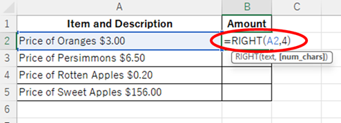
This time, as shown in the figure above, to extract 4 characters from the "A2" cell, set the "string" as the "A2" cell, and specify the number of characters as 4. Then, enter the following formula.
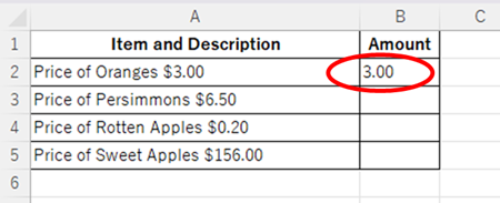
=RIGHT(A2,4)Then, the amount could be displayed as shown in the figure below.
However, when this function was also applied to the cells below, the "B4" cell displayed the characters to the left of the amount, while the "B5" cell showed only the last four digits, "6.00," of "156.00," as illustrated in the figure below.
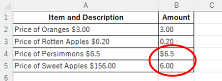
This is because the amount in each cell is not 4 characters but 3 digits in cell "B4" and 6 digits in cell "B5".
If the position of the character you want to extract is different in each cell, you can use the FIND function to fix this problem.
How to use the FIND function
The FIND function returns a number that tells you the position of a specific character or string in a cell.
=FIND(search string,target,[start position])
Both full-width and half-width characters are counted as one character.

To find the position of the "$" sign in cell "A2", enter the function as shown below.
=FIND("$",A2)The number "18" was returned as shown in the figure below.

This is because the "$" symbol is the 18th character from the left.
However, what we want to find out is how many characters are to the right of the "$" symbol.
To calculate this, use the LEN function.
How to use the LEN function
The LEN function is a function that can count the number of characters in a cell.
=LEN(string)
Both full-width and half-width characters are counted as one character.
To count the number of characters in cell A2, enter the following:
=LEN(A2)This returns the total number of characters in the cell, which is 22.
Using the above, you can calculate the number of characters to the right of the "$" sign as follows:
Number of characters in the cell (22) minus number of characters up to the "$" sign (18) equals the number of characters to the right of the "$" sign (4).
This calculation can be expressed with the following function
=LEN(A2)-FIND("$",A2)When this formula is reflected from "B2" cell to "B5" cell, the number of characters in the amount is reflected as shown in the figure below.
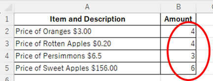
The following formula is the same as the first one when this function is reflected in the character count of the RIGHT function.
=RIGHT(A2,LEN(A2)-FIND("$",A2))When this formula is reflected from "B2" cell to "B5" cell, the amounts are reflected as shown in the figure below.
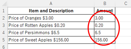
Summary
In this article, we explained how to extract the text to the right of a specific character. If you want to extract the text to the left of a specific character, please refer to the article titledHow to extract characters before a specific character "LEFT and FIND functions in Excel"article for more information.
For detailed usage of the RIGHT function, see the article "RIGHT and LEFT Functions to Extract a Specific Number of Characters from the Right or Left of a String in Excel".Excel RIGHT and LEFT functions to extract a specific number of characters from the right or left of a string*


Comment