Being able to use the VLOOKUP function will expand the range of data handling methods, and will help you to be seen as an intermediate Excel user from an Excel beginner. In this article, we will show you how to use the VLOOKUP function.
For the combination of the INDEX and MATCH functions, which compensate for the weaknesses of the VLOOKUP function, seeHow to use Excel (Excel) INDEX and MATCH functions in combination.
concrete example
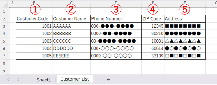
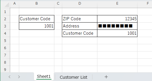
We have prepared this example.
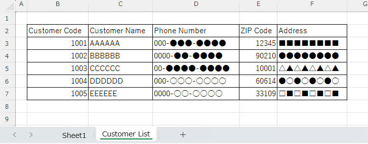
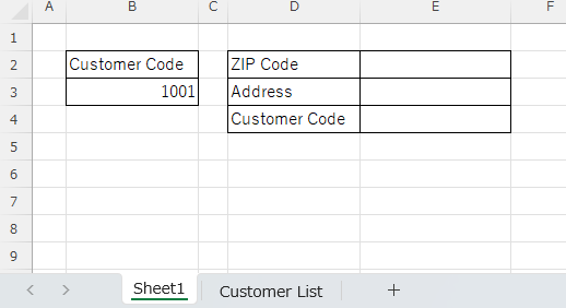
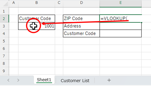
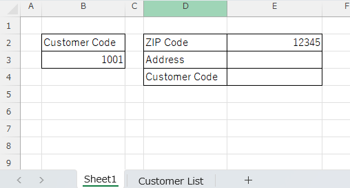
Then, by entering the customer code in the "B3" cell of the table shown below, I will extract the values from the customer master for the zip code, address, and customer name in the "E" column.
How to write VLOOKUP functions
VLOOKUP(search value,range,column number,[search method])
First, enter the following function in the 〒 (postal code) cell "E2" cell on the sheet you want to display.
=VLOOKUP($B$3,'Customer List'!$B$2:$F$7,4,0)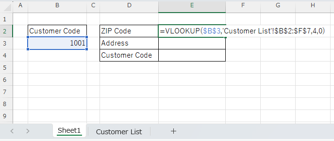
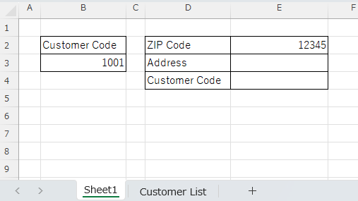
You can then display the zip code as follows.
This section explains the meaning of each item and how to enter the information.
search value
VLOOKUP(search valuerange,column number,[search method])
As the name implies, this is the key value you want to search for. The values of the rows that match this value can be extracted.
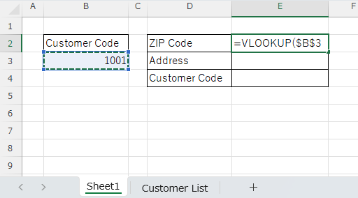
In this case, it is "B3" cell. In this case, the search value does not move from the "B3" cell to any other cell, so in order to make it an absolute reference, the "$B$It is convenient to use "3".
After entering up to =VLOOKUP( in the "E2" cell, click on the cell containing the customer code in "B3" and then press the "F4" key.

Then the input status is as shown in the figure below.
Scope.
VLOOKUP(searchvalue,Scope.column number,[search method])
Next is "scope. This refers to the scope of the database.
The input method is to hit a comma (,) after entering the search value and select the "Customer Master" sheet with the database in that state.
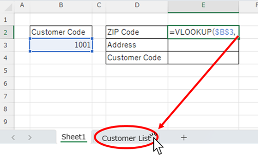
When the "Customer Master" sheet appears, specify a range for the entire data range.
At this time, the data range also does not move, so press the "F4" key for an absolute reference ($B$2:$f$7).
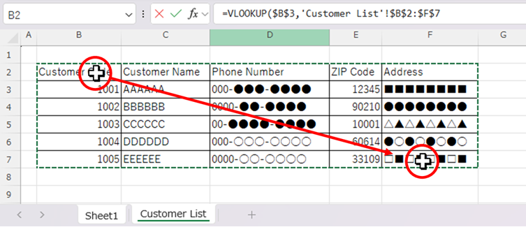
In this case, the first column must be the column where the "search value" (in this example, the customer code) is entered. Otherwise, you will not be able to search by the search value.
column number
VLOOKUP(searchvalue,range,.column number,[Search Methods])
Next is the column number. The column number specifies how many columns of the database the data to be extracted is in.
Since we want to extract "ZIP code" this time, the column number is "4".
To enter a range, hit a comma (,) after entering the range, and then use the numeric keypad to enter "4".
Search Method
VLOOKUP(searchvalue,range,columnnumber,.[Search method].)
Finally, there is the search method.
To enter the column number, hit a comma (,) after entering the column number, then use the numeric keypad to enter "0" and press "enter" key.
If the correct zip code is displayed in the "E2" cell in this state, you have succeeded.
TRUE" or "FALSE" is entered here, but since it is rarely necessary to specify anything other than "FALSE," it is safe to assume that "FALSE" is entered here.
TRUE" and "FALSE" can be replaced with "1" and "0" respectively.
The search method is an optional argument, but if "TRUE" is entered, information on unintentionally close cells will be displayed if there is no corresponding value. If "FALSE" is entered, an error value is returned if no value is found.
Therefore, be sure to enter "0" without omission to avoid displaying incorrect output results.
Copy function
Once the zip code function is complete, we can then copy this function down to the bottom.
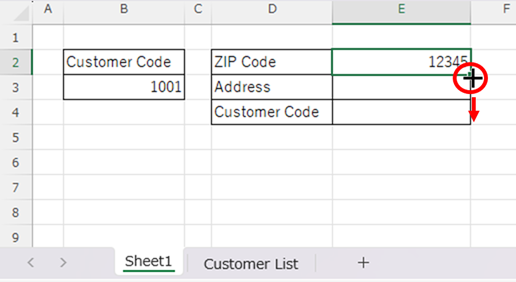
The function is created by absolute reference, so just copying down to the bottom will show the same value as the zip code.
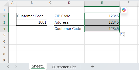
Therefore, change the "column number" of the function respectively, referring to the figure below.
=VLOOKUP($B$3,customer master!$B$2:$F$7,.4,0)
The address is 4→5
The name of the vendor is 4→2
If it looks like this, the function modification is complete.
Summary
The VLOOKUP function will not work unless the leftmost column in the database is the key column for the search value. Therefore, in this example, if there is data to the left of the customer code, the value cannot be extracted. I believe this is the greatest weakness of the VLOOKUP function.
This weakness can be compensated for by using the XLOOKUP function and the INDEX and MATCH functions; the XLOOKUP function cannot be used with Microsoft 365 Excel or versions older than Excel 2021, so to make it work on any computer I think the combination of the INDEX and MATCH functions is the best way for now.
How to use the combination of the INDEX and MATCH functions isHow to use Excel (Excel) INDEX and MATCH functions in combination.
I hope this article will be of help to you.


Comment