Error display "#DIV/0!" Meaning and Countermeasures Excel

Error messages are unavoidable when dealing with Excel, and you may be surprised when they suddenly appear, but there is nothing to fear if you know what they mean and what to do about them.

Here are the meanings of this error and countermeasures.

Meaning of "#DIV/0!

This comes up when "the denominator is a division of zero" or when there is "#DIV/0!" in the calculation target.

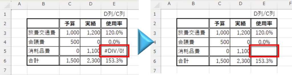
For example, assume the table below.

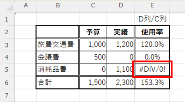
Column "C" shows the budget, "D" shows the actuals, and "E" shows the utilization rate as "actual divided by budget.

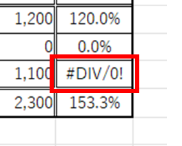
Here, the consumable expense usage rate in cell "E5" is showing the error "#DIV/0! This error is displayed because the formula is "1,100/0" and the denominator is zero.

Incidentally, the usage rate of meeting expenses in cell "E4" is "0÷500," which is not an error because the numerator is zero but the denominator is not.

Countermeasure 1: Replace errors with the "IFERROR function".

First, there is the ISERROR function that can be incorporated into the formula to prevent the error message from being displayed. This method allows the user to set the error message to a certain degree of freedom.

First, the top line containing the formula should read something like this

=IFERROR(D3/C3,"")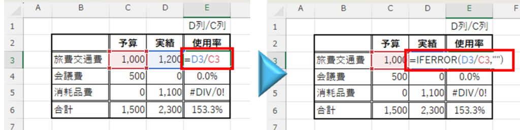

And this time, "" (blank) should be displayed for error values.

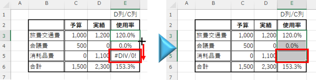
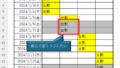
Next, with the cell where the formula was changed ("E3" cell) selected, move the mouse cursor to the lower right corner of the cell, the mouse cursor will change to a "+", and drag it to the last cell.

Then the value of cell "E5" changed to "blank" as shown in the figure above.

You can also display "-" (hyphen) instead of spaces by changing the function like this.

=IFERROR(D5/C5,."-")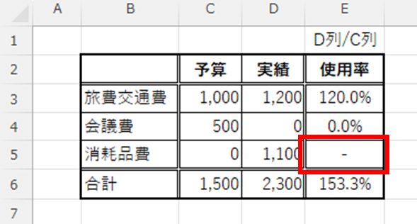

In addition, you can change the value to "0" zero, "100%" or any other value you like.

Countermeasure 2: Hide with "Conditional Formatting".

There is also a way to make error values invisible by setting "conditional formatting".

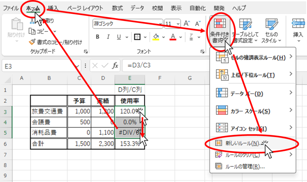
First select the range you want to format, then click on the "Home" tab, then "Conditional Formatting", then "New Rule".

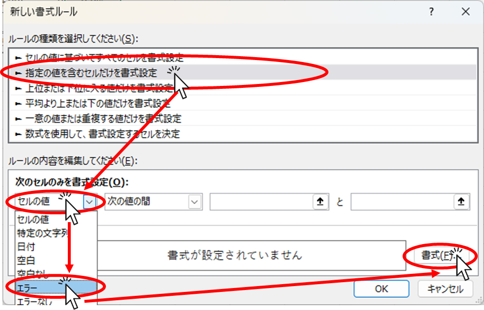
Select "Format only cells containing the specified value" from "Rule Type," change "Cell Value" to "Error," and click "Format."

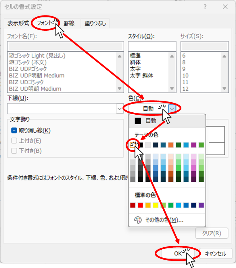
In the "Font" tab of the menu that appears, select "Color" the same color as the background. Usually, the color is "white," so "white" is selected here. Once the color is selected, click "OK.

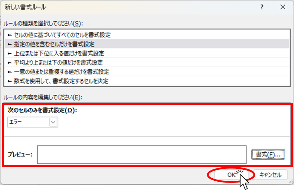
Confirm that the contents in the red frame are what you want to set and click "OK".

Now we have made the error value invisible. This is only invisible because the background and text colors are the same, but in reality the error value is still present here. Be careful if this cell is embedded in a formula.

Conclusion

1. #DIV/0!" is displayed when the denominator of the formula is "0
2. There are two ways to get around this: using the "IFERROR function" or using "conditional formatting".

Use different measures depending on how you use the table.