
Excel has a function to change the format according to cell values and various conditions. Here are some examples of specific settings.
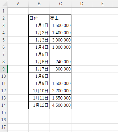
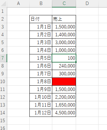
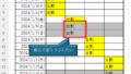
Suppose you have a simple table like the one below, and you want to shade in red the cells where no sales have been entered.
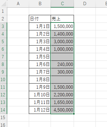
First, select the range you want to format.
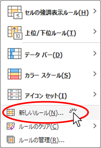
Then click on "Conditional Formatting" on the "Home" tab

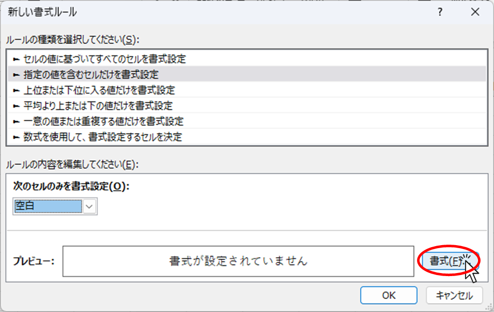
Then click on "New Rule
Click on "Format Only Cells Containing the Specified Value" and change "Cell Value" to "Blank".
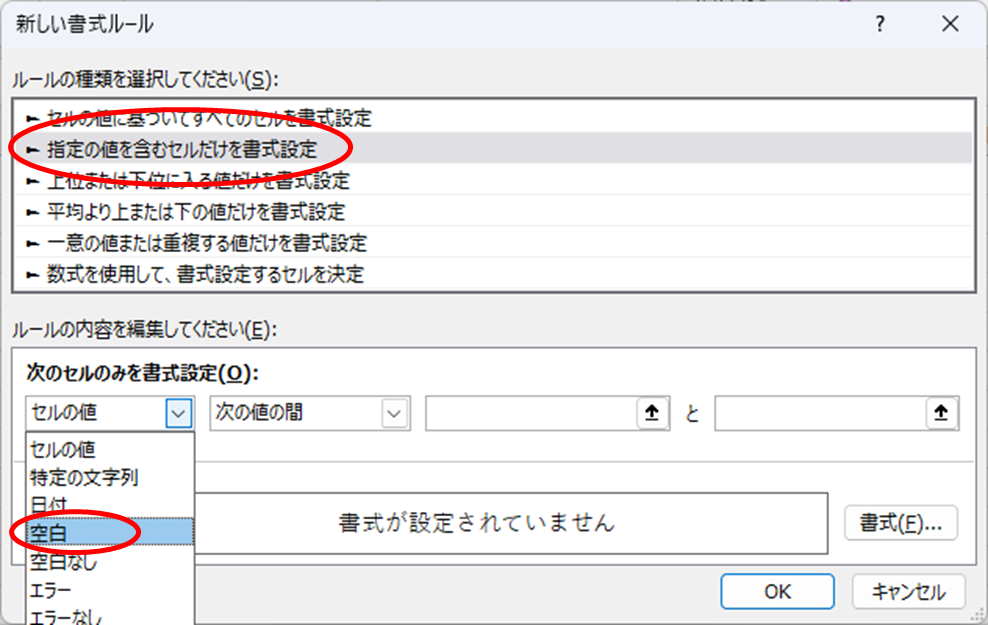
Then click on Format
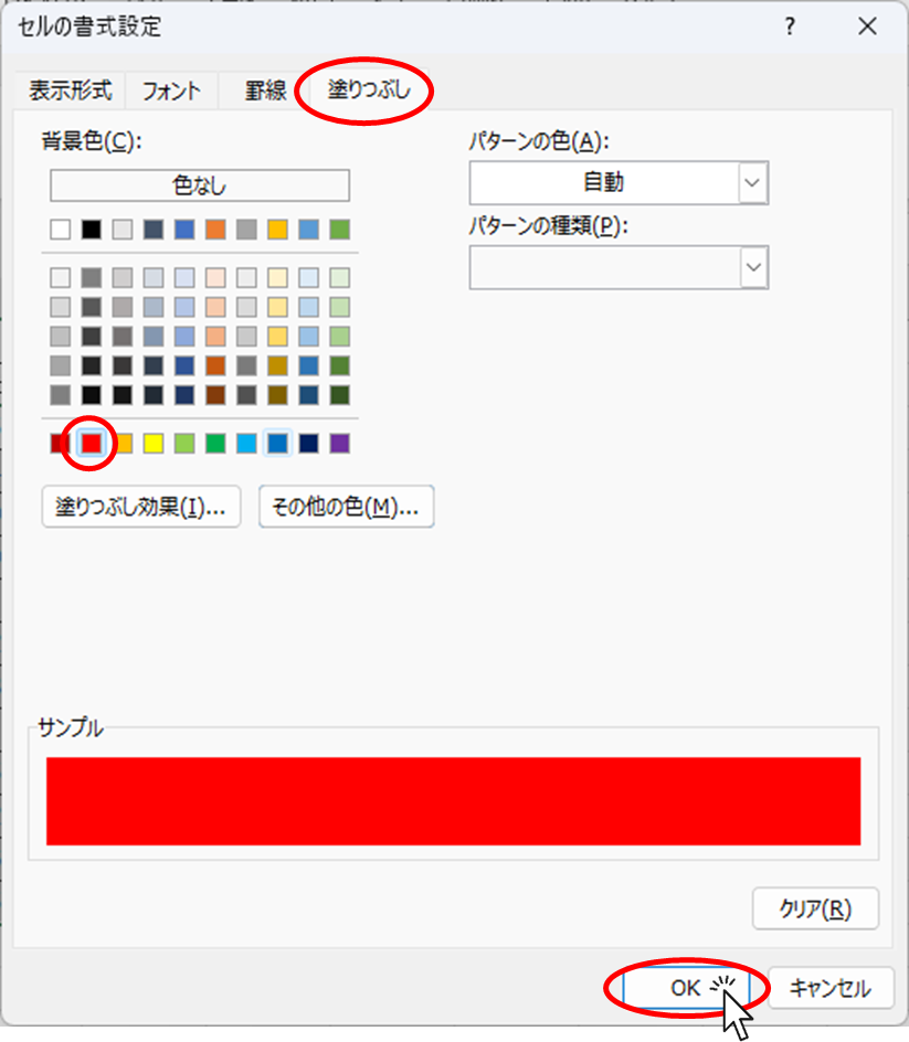
Change the settings to what you want in the displayed formatting screen and click the "OK" button.
This time we will fill in the blanks with red.
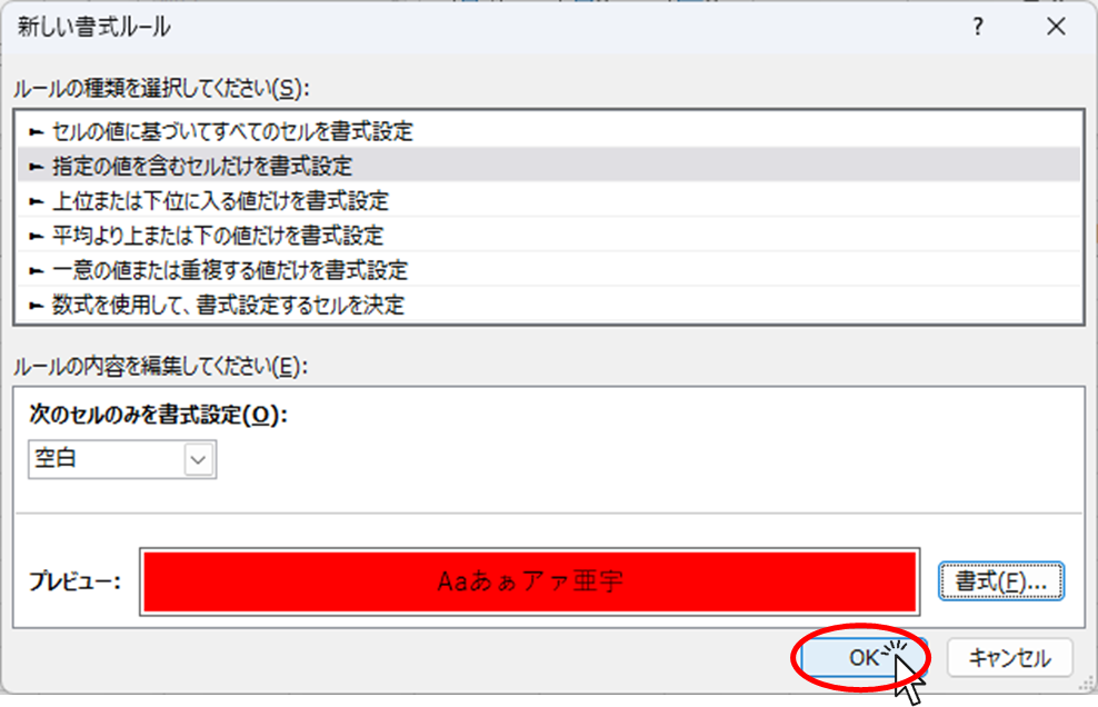
Click "OK
Then only the empty cells were filled in red.
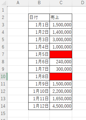
Try typing something into a blank cell in "C7"...
The red fill in cell "C7" has disappeared.


Comment