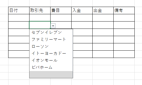
In the previous article, we introduced how to allow entering items that are not included in a dropdown list.
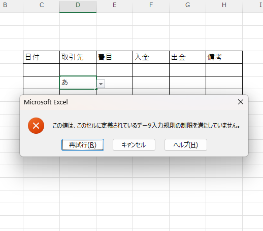
However, when you try to aggregate data using the VLOOKUP function or the INDEX/MATCH function, it won’t work properly unless there is an exact match.
In such cases, you can make it easy to identify which items were manually entered by changing only those cells’ colors.
For more information on dropdown lists, please also refer to this article.
Apply conditional formatting
For details on how to set up conditional formatting, please also refer to this article.
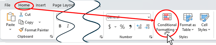
First, select one of the cells you want to apply ”Conditional Formatting” to.
Next, click [Conditional Formatting] on the [Home] tab.
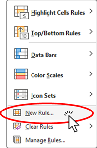
From the displayed menu, click [New Rule].
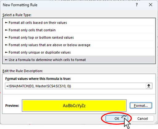
In the list of rule types, click Use a formula to determine which cells to format.
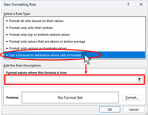
In the space provided below, enter the following formula:
=ISNA(MATCH(selected cell address, reference range for dropdown, 0))
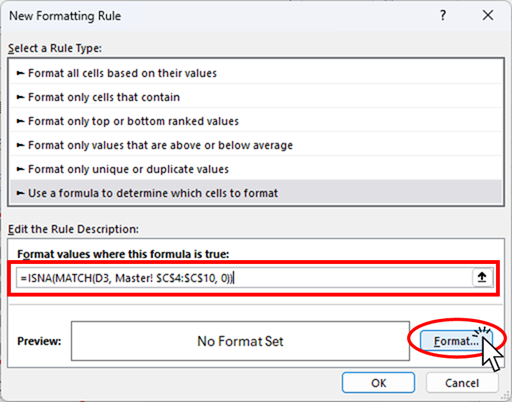
In this example, it is as follows:
=ISNA(MATCH(D3, Master! $C$4:$C$10, 0))Once the formula is entered, click [Format].
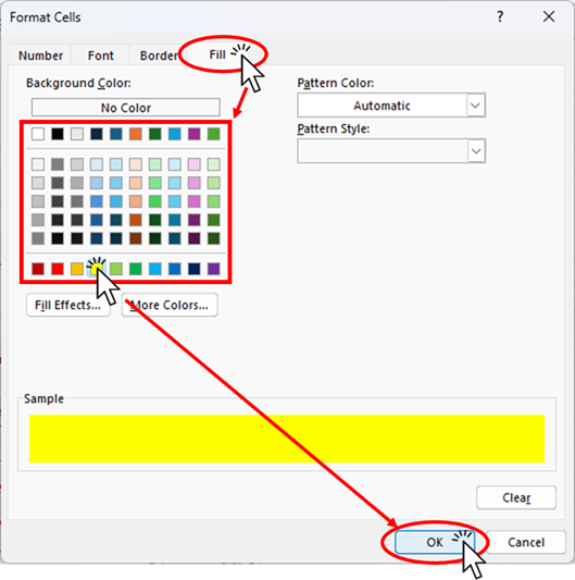
From the Fill tab in the displayed menu, choose your preferred color and click [OK].
Click [OK] again.
This completes the formatting for the initially selected cell "D3".
Copy the formatting
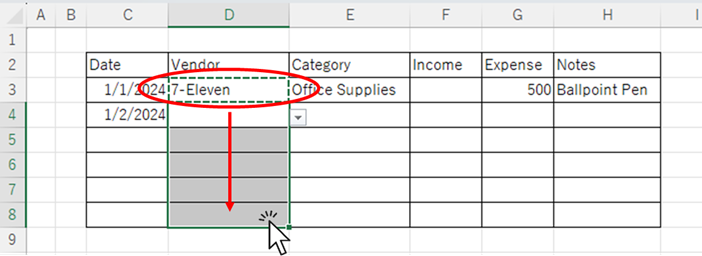
Next, copy the formatting to the remaining cells.
With cell D3 selected, press [Ctrl] + [C] to copy, then select cells D4 to D8 and right-click.
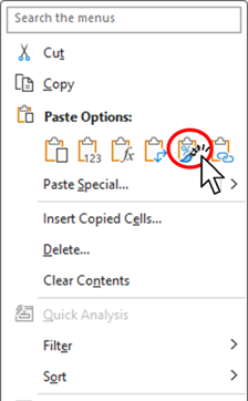
From the displayed menu under [Paste Options], click the [Formats button].
Now the formatting has been copied to the remaining cells.
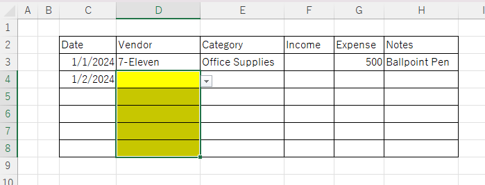
However, it seems that empty cells cannot be matched with the MATCH function, so as you can see, all empty cells have also turned yellow.
If you want to avoid coloring empty cells, you will need to add another condition to keep them white.
Conditional Formatting to Ignore Blank Cells
Select one of the cells you want to apply Conditional Formatting.
Next, click [Conditional Formatting] on the [Home] tab.
From the displayed menu, click [New Rule].
This time, in the list of rule types, click Format only cells that contain, then change the value type to Blanks.
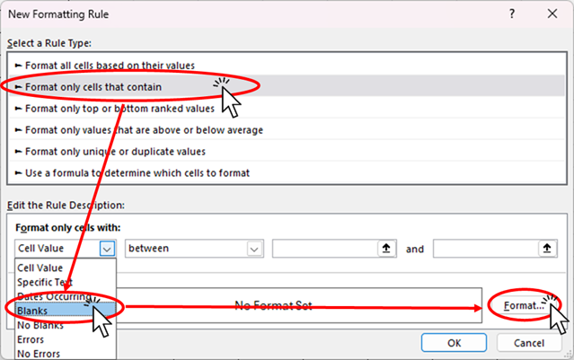
Once changed to blank, click [Format].
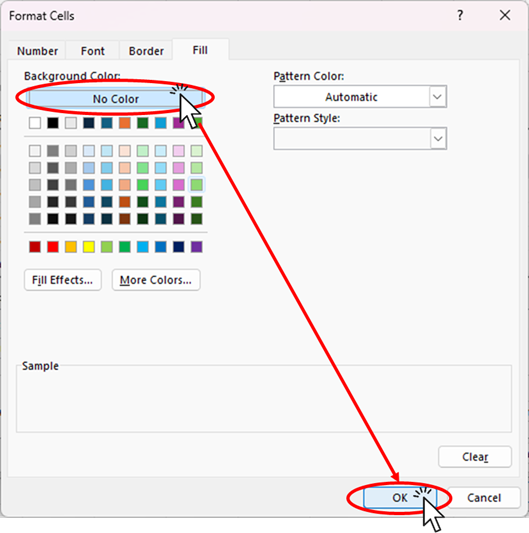
In the formatting menu, “No color” is likely selected by default, click “No color” again just to be sure, and then click OK.
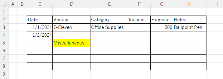
Finally, as before, copy the formatting from the formatted cell to the remaining cells.
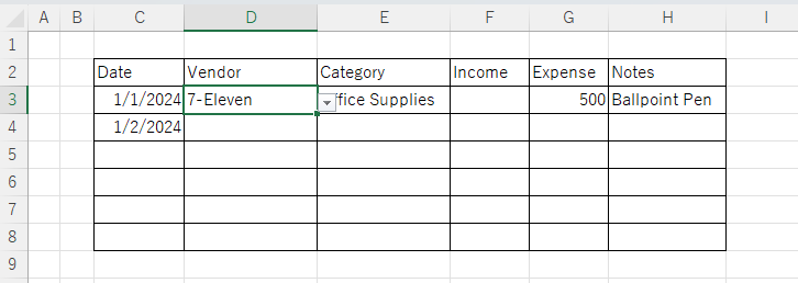
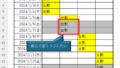
This completes the formatting. As you can see in the figure below, cells containing items from the list or blank cells remain white, while only cells where something else that are not in the list was entered are filled in yellow.
Summary
As mentioned above, if you use the VLOOKUP function or the INDEX/MATCH function to tabulate the data, it is not possible to tabulate the data well unless it is an exact match. Therefore, we always want the input value to be selected from a pull-down menu, but this may cause problems if there is no choice when inputting the data.
In such cases, it may be smoother to allow input of values not in the list and highlight them for later correction, as shown in this example. Pleases choose the method that helps you work most efficiently.
For how to set up a dropdown list, refer to this article:
For how to allow entering items not in the list in a dropdown, see this article:


Comment