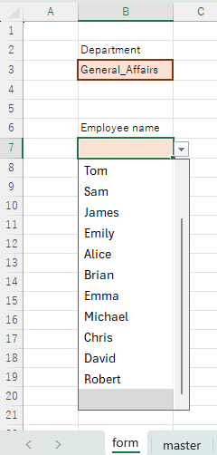
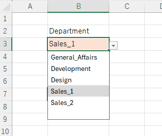
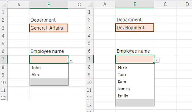
When you want to display a pull-down list of employee names, as in the image above, if all employees are displayed, the amount of information displayed is too large, and it is very inconvenient because it is not clear who is in which department.
In this case, it would be simpler and easier to use if you first select a department and only people in that department are displayed in the employee name pull-down.
Therefore, we will show you how to link the two pull-downs from major categories to minor categories.
Click here to see how to create a basic pulldown.Creating a pull-down (drop-down) Excel (Excel)
There are two main ways to link the two pull-downs: one pattern has the list of references in a single vertical column, and the other has the major categories in a table on the horizontal axis.
The latter is here.Linking two input rules without macros (to reflect on multiple lines) Excel (Excel)We will introduce the former method in this issue.
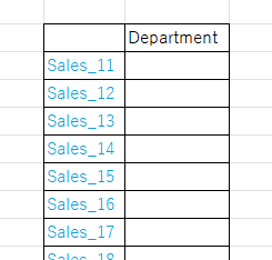
Create a list of major categories (departments)
First, create a list of departments.
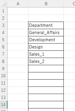
This needs no special explanation. Arrange the departments vertically in a row.
Create a list of subcategories (employee names)
Next, create an employee list.
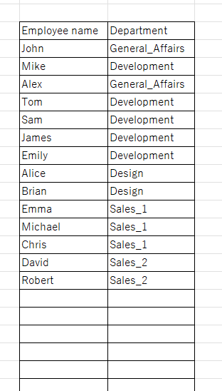
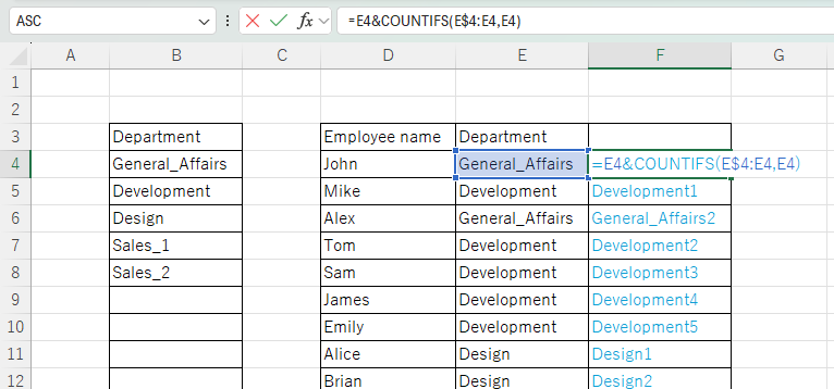
At this point, list the employee's department next to the employee's name. Make sure that the department names match exactly. If there is a space or a wrong half-size/full-width character, it will not be possible to refer to the employee's department.
Next, write a function like this next to the department.
=E4&COUNTIFS(E$4:E4,E4)At this time, pay attention to where the "$" mark is inserted.
Then copy this function to the bottom.
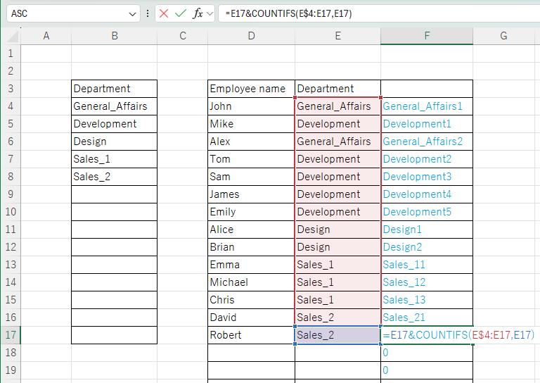
=E17&COUNTIFS(E$4:E17,E17)If the correct place to put the "$" mark when copied down to the bottom is in the correct place, the function will look like this.
What this function is doing is counting the number of people in the same department as this employee, including yourself. This allows us to number the departments sequentially from the top.
Create an input form
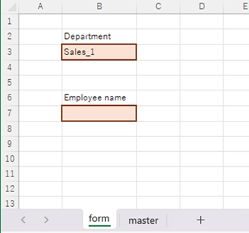
We will name the sheet "Form" and create a form there.
The department name is to be made in cell "B3".
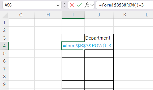
Create a pull-down reference list of subcategories
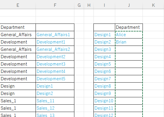
This time, in cell "I4" of the "Master" sheet
= Form!$B$3&ROW()-3The following is a description of the product.
The meaning of this function is to refer to the "B3" cell on the "Form" sheet by absolute reference to the department name, and to display the sequential number behind it, ROW() is used to subtract the number of rows, 3 since it is the fourth row, and the sequential number is 1.
Copy this function down to the bottom.
The bottom line here is that there are not originally several rows of data, so it is arbitrary to decide how many rows to create. The number of rows should be greater than the number of people in a department. If the number of rows is less than the number of people in the department, the last person in the department will not be able to be selected.
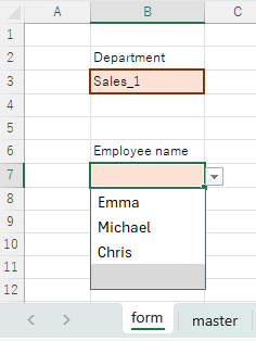
After copying the function down to the bottom, on the "Forms" sheet
If you select a department like this
This is how it appears on the "Master" sheet.
Then use the index match function on column J
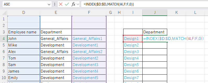
=INDEX(D:D,MATCH(I4,F:F,0))Describe it as such and copy it to the bottom.
Detailed usage of the index and match functions is explained here.How to use Excel (Excel) INDEX and MATCH functions in combination
Then it showed up like this in column J.
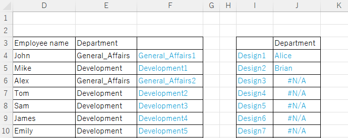
An error was displayed for data after "Design3" that did not exist in column F.
Therefore, each of the functions in column J is sandwiched between IFERROR functions and described like this.
=IFERROR(INDEX(D:D,MATCH(I4,F:F,0)),"")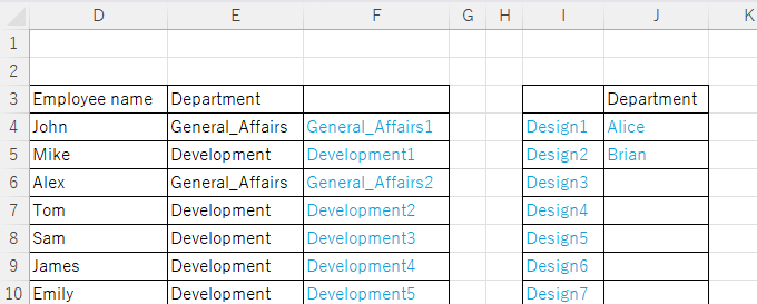
Now the rows that do not exist in column F will be blank, and the error disappears.
Set up a pull-down for employee names
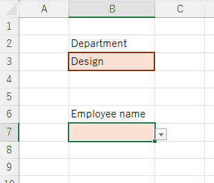
Finally, set the input rules for the employee name entry field on the "Form" sheet.
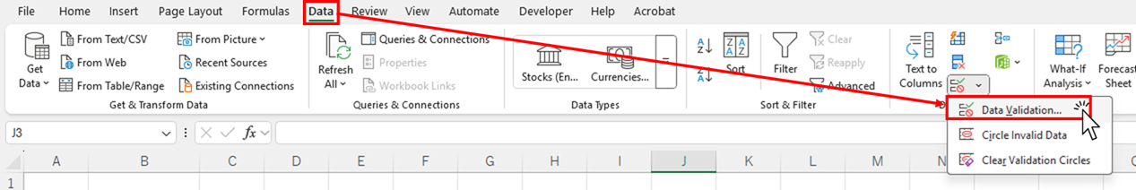
On the "Data" tab, click on "Data Entry Rules.
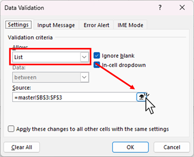
Change the input value type to "List" and specify the original range of values from this button.
Specify this part of the "master" sheet, in this example from J4 to the last row of column J, and press the "Enter" key.
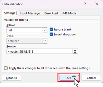
You will then be returned to this screen and click the "OK" button.
This completes the setup in which switching the "B3" cell causes the choices in the "B7" cell to be linked.
Advantages of this method
- Useful when the list of data to be linked is arranged vertically in a row
If there is a list of references to be presented separately, which is summarized in a tableLinking two input rules without macros (to reflect on multiple lines) Excel (Excel)table is more convenient, but if the data are arranged in a single column, it is necessary to rearrange them in a table.
- Easy maintenance of the master
If an employee moves departments in this example, maintenance is completed by simply changing the department item for that employee in the pull-down menu.
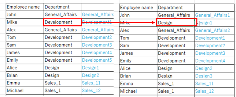
For example, if Mr. Mike is transferred from the Development Department to the Design Department, simply correct the department column in the employee list.
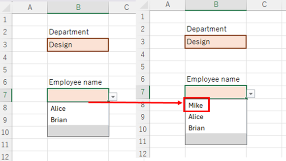
You can change the choices that appear in the employee name.
If it is in a table, both tables must be corrected, which increases the man-hours involved and makes it easier for errors to occur.
Disadvantages of this method
- Cannot be used to link multiple lines
The biggest disadvantage is this. In this example, there is only one row of cells to be linked in the work sheet, but if you want to link each row individually, it is not feasible unless you use a macro. If you want to use it in such a way, you have to use the case of a table.
- Complicated to make
This is also a major disadvantage, but it is difficult to create without some knowledge of functions, and it is a little complicated because it is made by combining many functions.


Comment