
Many companies, both general corporations and sole proprietorships, use petty cash to carefully manage the flow of money for both personal and business finances.
However, tasks such as carefully reconciling balances and transferring the contents of the cash book to the accounting system are very time-consuming and prone to errors, resulting in a lot of wasted man-hours.
This time, we're going to create such a petty cash book in Excel and build a system to automatically import it into our accounting system at the end.
Make it from its appearance
You're probably in a state of not knowing where to start. In that case, I recommend starting with the appearance, as it will be easier to understand what you need next.
Create input fields
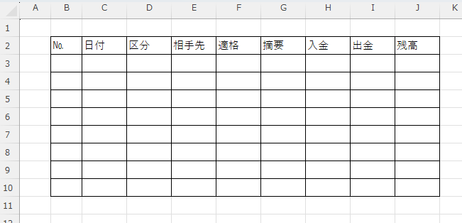
First, I'll write down the input fields that seem necessary.
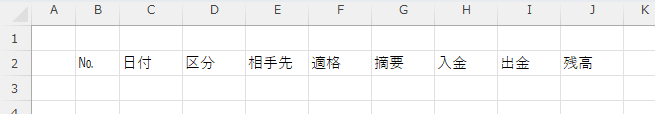
You can freely add or rearrange items as you create them, so let's start by writing down whatever comes to mind.
Draw a line
First, specify the range for the "columns" to include all items in the header row, and then specify the range down to the "rows" a little below.
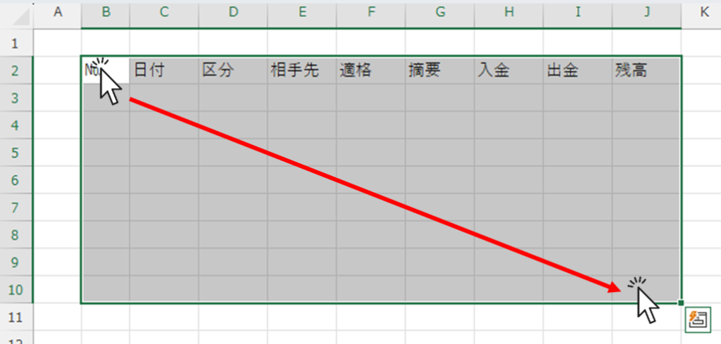
We can make adjustments here later as well, so I'll just put in some placeholder lines for now.
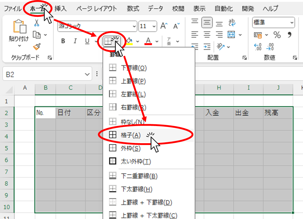
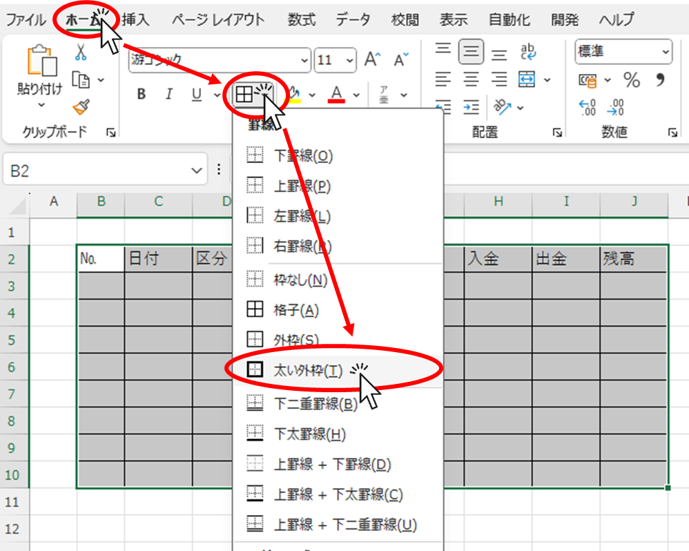
Next, click "Home" tab -> "Borders" -> "Grid".
I've managed to create a simple "grid" so far.
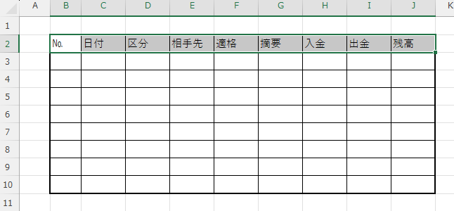
Click to select "Thick Outer Frame" in a similar range.
This time, I will select only the title row in the first line.
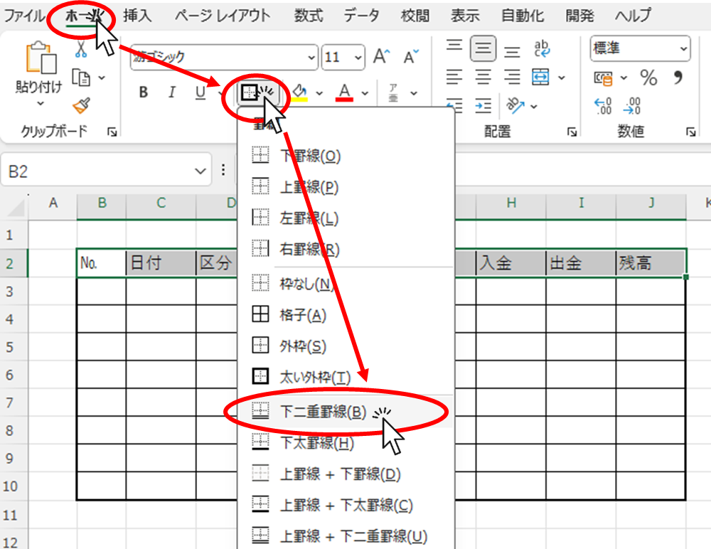
In this state, click "Double underline" this time.
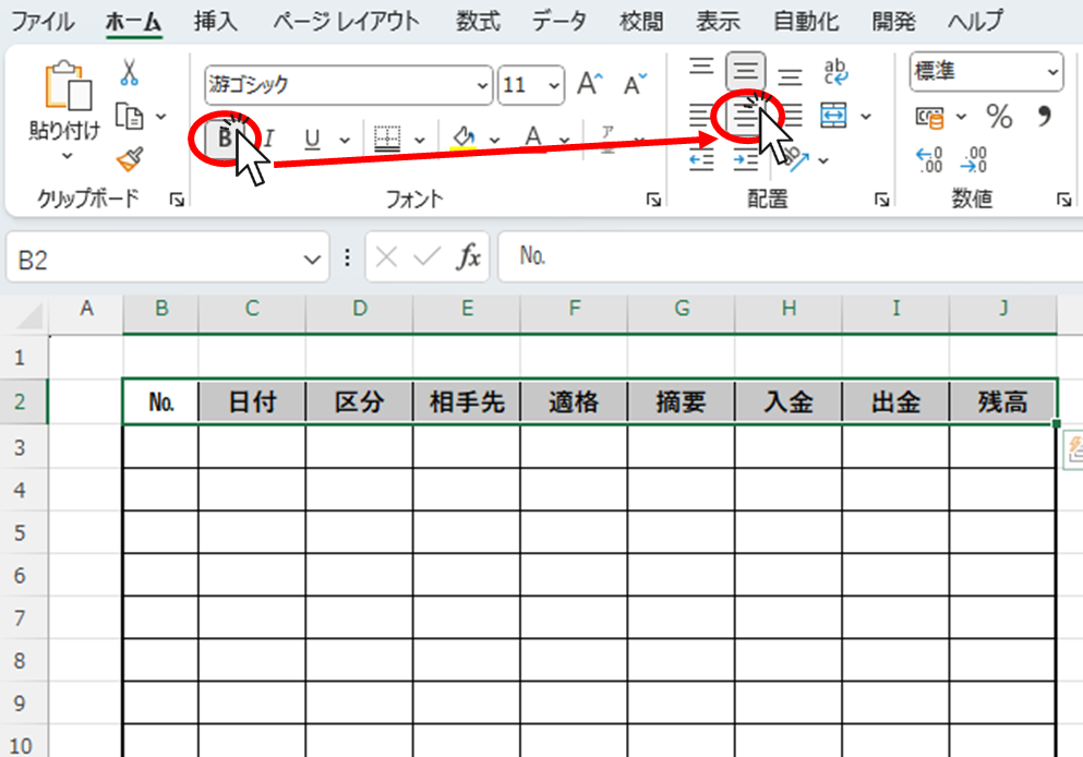
Without changing the selection, please click "Bold" and "Center align" as shown in the diagram above.
Adjust column width
To make it easier to understand, I'll add some sample data to lines 1 and 2.
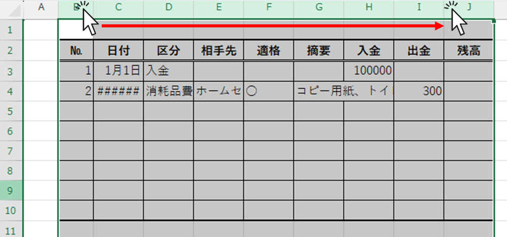
Then, select columns B through J.
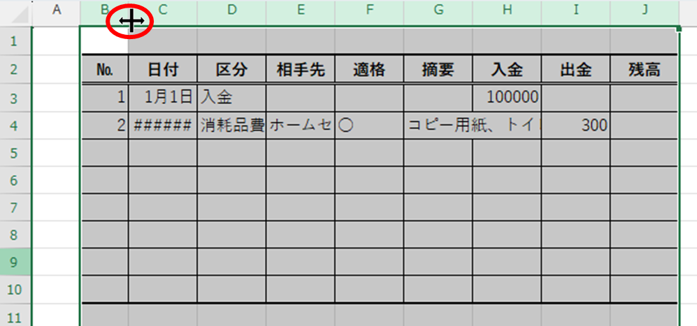
Then, if you move the mouse cursor between columns, such as between column B and column C, the mouse cursor will change shape as shown in the figure above. Double-click while in this state.
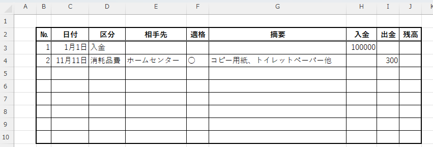
It's starting to look convincing all of a sudden.
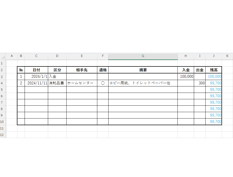
Enter calculation formula
Next, enter the following in cell "J4". The key point is that it is the second row of the row where data is being entered.
=J3+H4-I4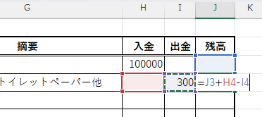
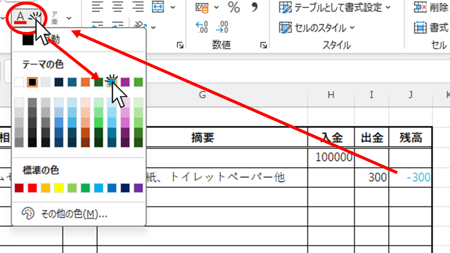
And this is my preference, but I make the text color of cells containing formulas blue. This makes it immediately obvious and easier to understand which cells contain numbers directly and which contain formulas.
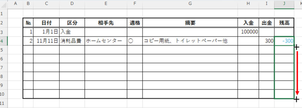
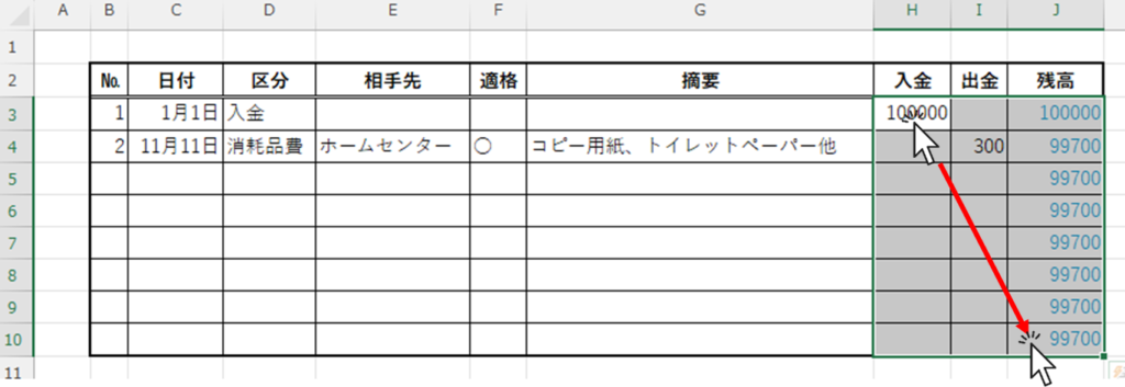
Now, if you move your mouse cursor to the bottom right corner of the cell where you entered the function, the cursor will change to a "+" shape. Drag this down to the bottom of the table.
Similarly, now copy it upwards.
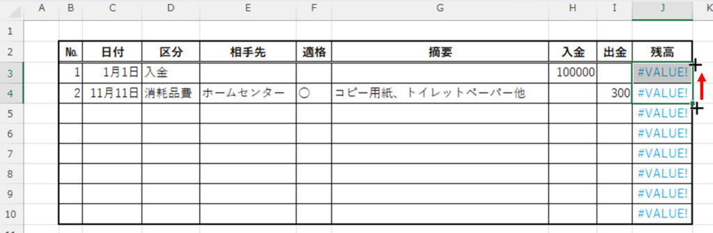
Then, suddenly, the entire screen was filled with the error message "#VALUE!".
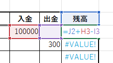
This is an error because the cells intended for addition in the entered formula contain the string "Balance" instead of numbers, making calculation impossible. The reason I entered the function starting from the second row previously was to confirm if the formula was entered correctly, as I knew it would result in an error if entered in the first row.
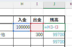
Then, delete the "J2" part from cell "J3".
=H3-I3And that's it. I believe the error message should disappear now.
Format input values
If it remains as is, the amount will be difficult to read without commas, so select the entire area where the amount is entered and format it.
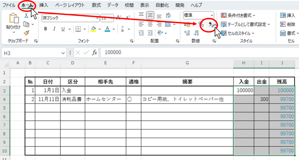
Click "Comma Style" in the "Home" tab.
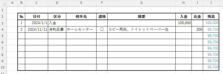
After that, feel free to format it to your liking. By the way, I centered columns B and F, and changed column C (dates) to a short date format.
Summary
- Let's start with the appearance.
- Insert dummy data
- Enter calculation formula
- Adjust the formatting for better readability
The visual adjustments are now complete.
Next time, I'll try to make it easier to select from a dropdown and to input things.


Comment