
As you can see in the example below, when extra data appears after the main text, you can’t just use the LEFT function to pull out the string. That’s because the length of the text isn’t always the same.
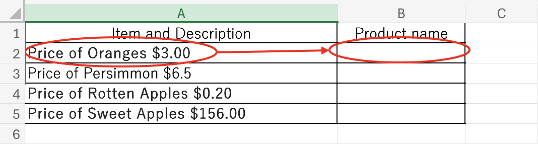
To extract the part that starts withA2for example the cell containing$3.00, you can use a function to get the text on the left side of the "+" sign.
=LEFT(A2,FIND("\",A2)-1)In the next sections, we will explain how this function works.
To extract the characters before a specific character, use theHow to Extract Text After a Specific Character in Excel Using RIGHT and FIND.
How to use the LEFT function
The LEFT function is used to extract a certain number of characters from the left side of a cell’s text.
=LEFT(string,[number of characters])
Both full-width and half-width characters are counted as one character.
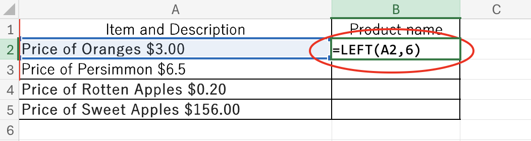
This time, in the situation shown in the above figure, the "A2cell to the left of the6To extract a string of characters, the "string" must be "A2cell, the "number of characters" is6characters, so enter the following
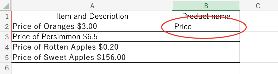
=LEFT(A2,6)Then, as shown in the figure below, we can now display the text without the monetary values.
However, when we apply this function to the cells below, it always extracts only six characters. As a result, some prices are cut off, and the full text cannot be displayed.
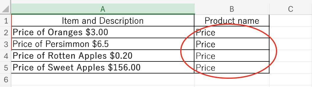
This happens because the text in each cell is not always six characters long.
If the position of the character you want to extract is different in each cell, you can use the FIND function to fix this problem.
How to use the FIND function
The FIND function returns a number that tells you the position of a specific character or string in a cell.
=FIND(search string,target,[start position])
Both full-width and half-width characters are counted as one character.
To find the position of the "$" sign in cell "A2" enter the function as shown below.
=FIND("$",A2)The number "18" was returned as shown in the figure below.
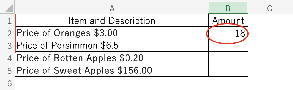
This is called "$3.00This is because the "+" mark is the "seventh letter" counting from the left.
To reflect this in the LEFT function, the function is described as follows.
=LEFT(A2,FIND("\",A2))Then you can see the following "$3.00I even saw the "" mark.
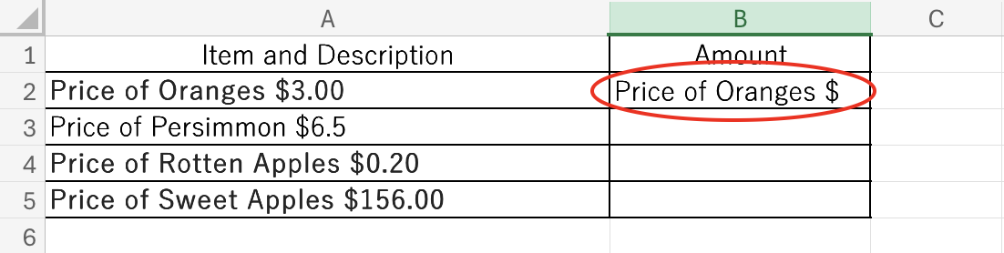
This is a$3.00This is because the "" mark is the seventh character and the seventh character from the left is displayed.
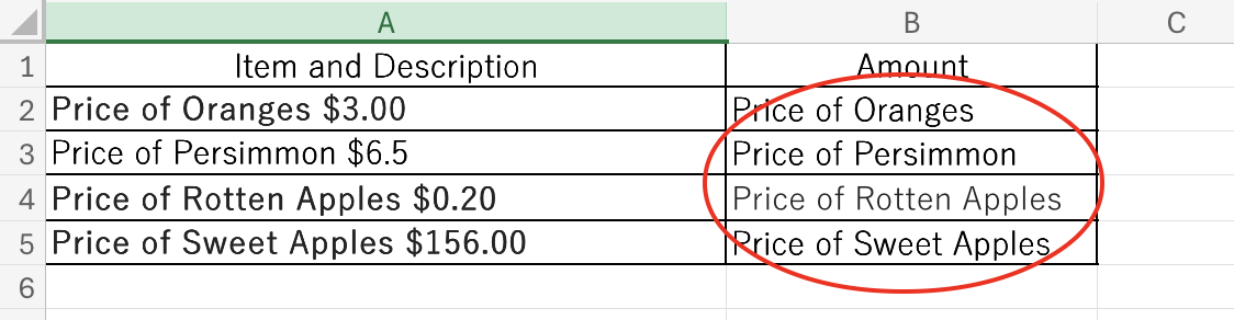
To avoid this, the FIND function is followed by "-1I will try to describe "the
=LEFT(A2,FIND("\",A2))-1)When this is reflected from "B2" cell to "B5" cell, it can be displayed correctly according to the number of characters as shown in the figure below.
Summary
In this article, we explained how to extract the text to the left of a specific character. If you want to extract the text to the right of a specific character, you can use theHow to Extract Text After a Specific Character in Excel Using RIGHT and FINDarticle for more information.
The usage of the LEFT function isExcel RIGHT and LEFT functions to extract a specific number of characters from the right or left of a string*


Comment