The SUMIF function can change the contents of the total according to the conditions, and the SUMIFS function can specify multiple conditions. We will explain why and how to use them in the following order: SUMIF function explanation → SUMIFS function explanation → Why you do not need to use the SUMIF function...
SUMIF Function
I will start with the SUMIF function, which I said you don't have to use.
How to write the SUMIF function
- =SUMIF(range,search condition,[total range])
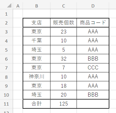
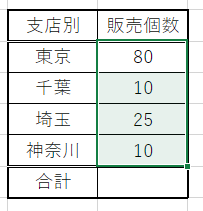
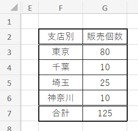
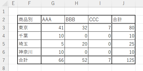
First, let us assume that we have the above data. Think of it as the number of units sold in a given month at the Tokyo, Chiba, Saitama, and Kanagawa branches.

Next, I would like to create a list of units sold by branch as shown above.
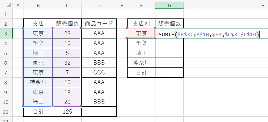
The "range" to search is from B3 to B10, which contains the branch name, so "B3 to B10" is the "range" to search.$B$3:$B$10"
Since "Search Criteria" is F3, you can use the "Search" button.$F3"
The "total range" is C3~C10, which contains the number of units sold.$C$3:$C$10"
Put this in the top "G3" cell.
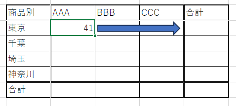
=SUMIF($B$3:$B$10,$F3,$C$3:$C$10)Enter
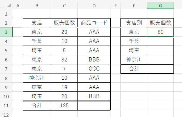
The total number of units sold in Tokyo was entered as shown above.
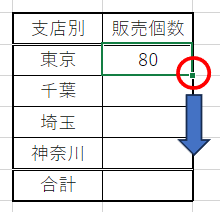

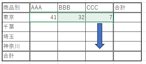
Next, with the "G3" cell where you just entered the function selected, drag the lower right portion down with the mouse.
The function would then automatically populate and display the totals for each branch.
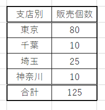
Finally, the SUM function is inserted into the total row and we are done.
SUMIFS Function
How to write the SUMIFS function
- =SUMIFS(total target range,condition range1,condition1,condition range2,condition2,...)

The data to be used is from the same table used when explaining the SUMIF function.
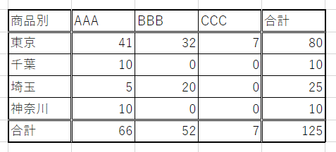
Next, I would like to create a list of units sold by branch and by product as shown above.
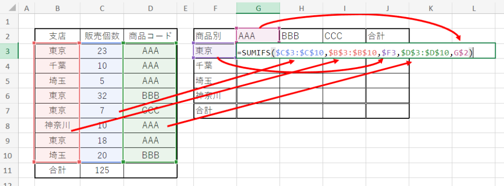
The "total range" is C3~C10, which contains the number of units sold.$C$3:$C$10"
Since "condition range 1" is from B3 to B10 where the branch name is written, you can use the "condition range 2" to specify the branch name.$B$3:$B$10"
Condition 1" wants to specify F3, so we can use "$F3"
Since "Condition range 2" is D3 to D10, which contains the product code, "D3" is the "condition range 1".$D$3:$D$10"
For "Condition 2," we want to specify G2, so we use "G$2"
Put this in the "G3" cell.
=SUMIFS($C$3:$C$10,$B$3:$B$10,$F3,$D$3:$D$10,G$2)Enter
Once entered, copy the function as above.
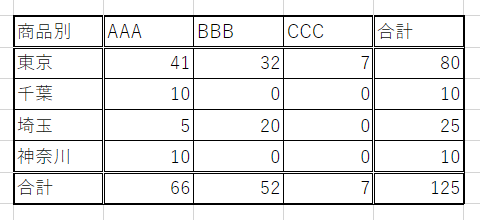
Finally, enter the total field to complete the process.
Why you should not use the SUMIF function
First, the SUMIFS function can be used with a single condition.

The function to be entered in the "G1" cell in Table 1 has only one search condition, but let's write it in the SUMIF and SUMIFS functions, respectively.
=SUMIF($B$3:$B$10,$F3,$C$3:$C$10)=SUMIFS($C$3:$C$10,$B$3:$B$10,$F3)The number of items entered is the same, but how differently they are arranged.
If, after creating Table 1 by branch, you want to look at the products, you can simply add more columns to the table, but you will need to change the conditions of the function.
- To convert a SUMIF function to a SUMIFS function and add a condition
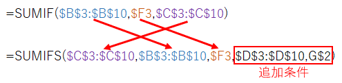
The function conversion is complicated by the need to sort items from the SUMIF function.
- To add a condition to the SUMIFS function
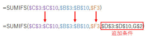
If you just want to add a condition to the SUMIFS function, you can process it by simply adding additional conditions behind it.
In other words, even if there is only one condition, if the SUMIFS function is used from the beginning, it is easy to add additional conditions later and mistakes are unlikely to occur. There is no merit in using the SUMIFS function.
We strongly recommend using the SUMIFS function even in situations where there is only one search condition.

Comment